Machine Learning Visualization

This example demonstrates a simple machine learning workflow with visualization. The Marimo version allows interactive parameter tuning and real-time updates.

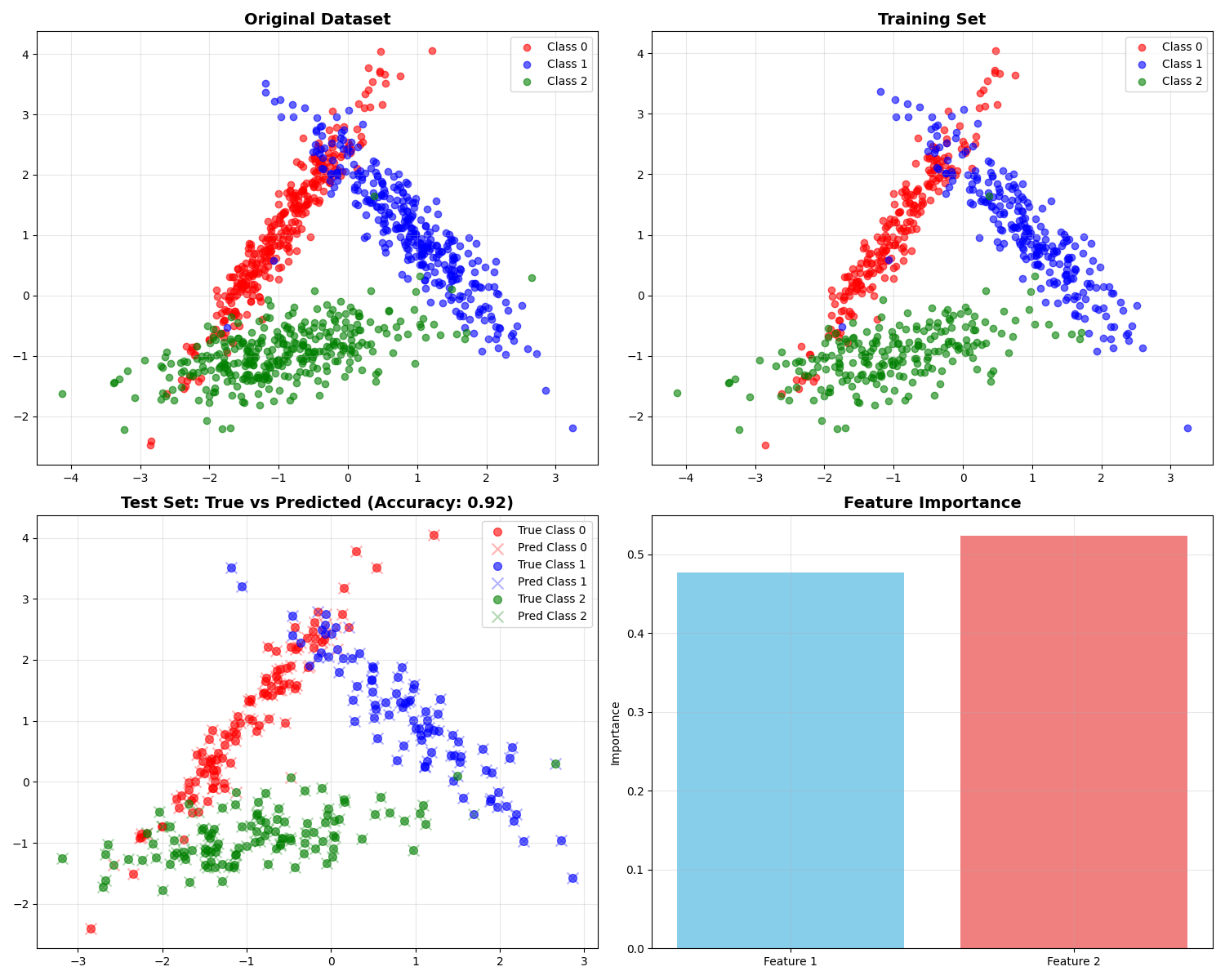
Generating synthetic classification dataset...
Training Random Forest classifier...

=== Model Performance ===
Accuracy: 0.920
Feature Importances:
  Feature 1: 0.477
  Feature 2: 0.523

Detailed Classification Report:
              precision    recall  f1-score   support

           0       0.87      0.93      0.90       101
           1       0.95      0.87      0.91        87
           2       0.95      0.95      0.95       112

    accuracy                           0.92       300
   macro avg       0.92      0.92      0.92       300
weighted avg       0.92      0.92      0.92       300


🚀 Launch in Marimo to:
   • Adjust model parameters interactively
   • Try different algorithms
   • Modify dataset parameters
   • See real-time performance updates

import matplotlib.pyplot as plt
import numpy as np
from sklearn.datasets import make_classification
from sklearn.model_selection import train_test_split
from sklearn.ensemble import RandomForestClassifier
from sklearn.metrics import accuracy_score, classification_report

# Generate synthetic dataset
print("Generating synthetic classification dataset...")
X, y = make_classification(
    n_samples=1000,
    n_features=2,
    n_redundant=0,
    n_informative=2,
    n_clusters_per_class=1,
    n_classes=3,
    random_state=42
)

# Split the data
X_train, X_test, y_train, y_test = train_test_split(
    X, y, test_size=0.3, random_state=42
)

# Train model
print("Training Random Forest classifier...")
model = RandomForestClassifier(n_estimators=100, random_state=42)
model.fit(X_train, y_train)

# Make predictions
y_pred = model.predict(X_test)
accuracy = accuracy_score(y_test, y_pred)

# Create visualization
fig, ((ax1, ax2), (ax3, ax4)) = plt.subplots(2, 2, figsize=(15, 12))

# Original dataset
colors = ['red', 'blue', 'green']
for i, color in enumerate(colors):
    mask = y == i
    ax1.scatter(X[mask, 0], X[mask, 1], c=color, alpha=0.6, label=f'Class {i}')
ax1.set_title('Original Dataset', fontsize=14, fontweight='bold')
ax1.legend()
ax1.grid(True, alpha=0.3)

# Training set
for i, color in enumerate(colors):
    mask = y_train == i
    ax2.scatter(X_train[mask, 0], X_train[mask, 1], c=color, alpha=0.6, label=f'Class {i}')
ax2.set_title('Training Set', fontsize=14, fontweight='bold')
ax2.legend()
ax2.grid(True, alpha=0.3)

# Test set with predictions
for i, color in enumerate(colors):
    mask = y_test == i
    ax3.scatter(X_test[mask, 0], X_test[mask, 1], c=color, alpha=0.6,
               marker='o', s=50, label=f'True Class {i}')

    mask_pred = y_pred == i
    ax3.scatter(X_test[mask_pred, 0], X_test[mask_pred, 1], c=color, alpha=0.3,
               marker='x', s=100, label=f'Pred Class {i}')

ax3.set_title(f'Test Set: True vs Predicted (Accuracy: {accuracy:.2f})',
              fontsize=14, fontweight='bold')
ax3.legend()
ax3.grid(True, alpha=0.3)

# Feature importance
feature_names = ['Feature 1', 'Feature 2']
importances = model.feature_importances_
ax4.bar(feature_names, importances, color=['skyblue', 'lightcoral'])
ax4.set_title('Feature Importance', fontsize=14, fontweight='bold')
ax4.set_ylabel('Importance')
ax4.grid(True, alpha=0.3)

plt.tight_layout()
plt.show()

# Print results
print("\n=== Model Performance ===")
print(f"Accuracy: {accuracy:.3f}")
print(f"Feature Importances:")
for name, importance in zip(feature_names, importances):
    print(f"  {name}: {importance:.3f}")

print(f"\nDetailed Classification Report:")
print(classification_report(y_test, y_pred))

print("\n🚀 Launch in Marimo to:")
print("   • Adjust model parameters interactively")
print("   • Try different algorithms")
print("   • Modify dataset parameters")
print("   • See real-time performance updates")