Meta Models

Certain models in scikit-lego are meta. Meta models are models that depend on other estimators that go in and these models will add features to the input model.

One way of thinking of a meta model is to consider it to be a way to decorate a model.

This part of the documentation will highlight a few of them.

Thresholder

The Thresholder can help tweak recall and precision of a model by moving the threshold value of predict_proba.

Commonly this threshold is set at 0.5 for two classes. This meta-model can decorate/wrap an estimator with two classes such that the threshold moves.

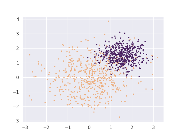
We demonstrate how that works below. First we'll import the necessary libraries and generate a skewed dataset.

Skewed dataset

import matplotlib.pylab as plt
import seaborn as sns

sns.set_theme()
cmap=sns.color_palette("flare", as_cmap=True)

import pandas as pd
import numpy as np
from sklearn.pipeline import Pipeline
from sklearn.datasets import make_blobs
from sklearn.model_selection import GridSearchCV
from sklearn.linear_model import LogisticRegression
from sklearn.metrics import precision_score, recall_score, accuracy_score, make_scorer

from sklego.meta import Thresholder

X, y = make_blobs(1000, centers=[(0, 0), (1.5, 1.5)], cluster_std=[1, 0.5])
plt.scatter(X[:, 0], X[:, 1], c=y, s=5, cmap=cmap);

Next we'll make a cross validation pipeline to try out this thresholder.

Cross validation pipeline

# %%time

pipe = Pipeline([
    ("model", Thresholder(LogisticRegression(solver="lbfgs"), threshold=0.1))
])

mod = GridSearchCV(
    estimator=pipe,
    param_grid={"model__threshold": np.linspace(0.1, 0.9, 500)},
    scoring={
        "precision": make_scorer(precision_score),
        "recall": make_scorer(recall_score),
        "accuracy": make_scorer(accuracy_score)
    },
    refit="precision",
    cv=5
)

_ = mod.fit(X, y)

CPU times: user 15.4 s, sys: 63.3 ms, total: 15.4 s
Wall time: 15.4 s

With this cross validation trained, we'll make a chart to show the effect of changing the threshold value.

Threshold chart

(pd.DataFrame(mod.cv_results_)
 .set_index("param_model__threshold")
 [["mean_test_precision", "mean_test_recall", "mean_test_accuracy"]]
 .plot(figsize=(16, 6)));

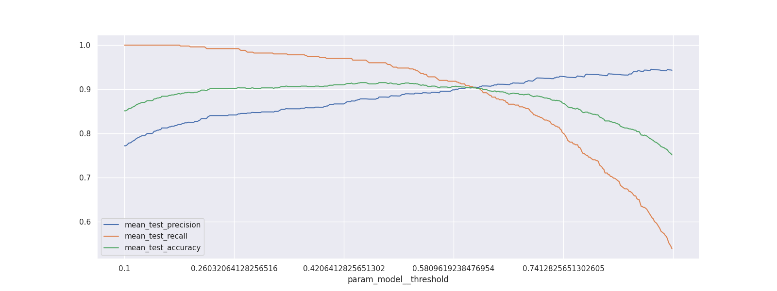
Increasing the threshold will increase the precision but as expected this is at the cost of recall (and accuracy).

Saving Compute

Technically, you may not need to refit the underlying model that the Thresholder model wraps around.

In those situations you can set the refit parameter to False. If you've got a predefined single model and you're only interested in tuning the cutoff this might make everything run a whole lot faster.

Cross validation pipeline - no refit

# %%time

# Train an original model
orig_model = LogisticRegression(solver="lbfgs")
orig_model.fit(X, y)

# Ensure that refit=False
pipe = Pipeline([
    ("model", Thresholder(orig_model, threshold=0.1, refit=False))
])

# This should now be a fair bit quicker.
mod = GridSearchCV(
    estimator=pipe,
    param_grid = {"model__threshold": np.linspace(0.1, 0.9, 50)},
    scoring={
        "precision": make_scorer(precision_score),
        "recall": make_scorer(recall_score),
        "accuracy": make_scorer(accuracy_score)
    },
    refit="precision",
    cv=5
)

_ = mod.fit(X, y);

CPU times: user 918 ms, sys: 0 ns, total: 918 ms
Wall time: 917 ms

Grouped Prediction

To help explain what it can do we'll consider three methods to predict the chicken weight.

The chicken data has 578 rows and 4 columns from an experiment on the effect of diet on early growth of chicks. The body weights of the chicks were measured at birth and every second day thereafter until day 20. They were also measured on day 21. There were four groups on chicks on different protein diets.

Setup

Let's first load a bunch of things to do this.

Setup

import numpy as np
import pandas as pd
import matplotlib.pylab as plt
from sklearn.linear_model import LinearRegression
from sklearn.pipeline import Pipeline, FeatureUnion
from sklearn.preprocessing import OneHotEncoder, StandardScaler
from sklearn.metrics import mean_absolute_error, mean_squared_error

from sklego.datasets import load_chicken
from sklego.preprocessing import ColumnSelector

def plot_model(model):
    df = load_chicken(as_frame=True)

    _ = model.fit(df[["diet", "time"]], df["weight"])
    metric_df = (df[["diet", "time", "weight"]]
        .assign(pred=lambda d: model.predict(d[["diet", "time"]]))
    )

    metric = mean_absolute_error(metric_df["weight"], metric_df["pred"])

    plt.figure(figsize=(12, 4))
    plt.scatter(df["time"], df["weight"])
    for i in [1, 2, 3, 4]:
        pltr = metric_df[["time", "diet", "pred"]].drop_duplicates().loc[lambda d: d["diet"] == i]
        plt.plot(pltr["time"], pltr["pred"], color=".rbgy"[i])
    plt.title(f"linear model per group, MAE: {np.round(metric, 2)}");

This code will be used to explain the steps below.

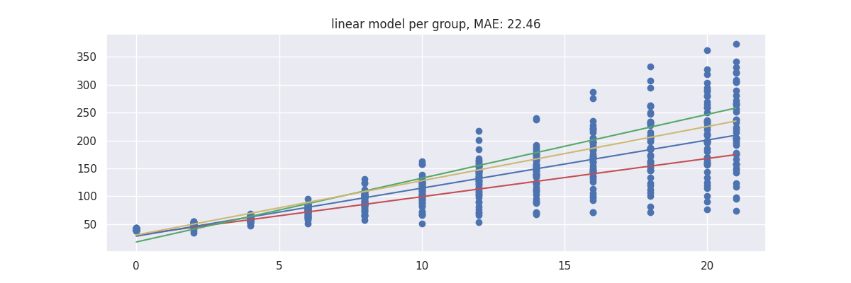
Model 1: Linear Regression with Dummies

First we start with a baseline. We'll use a linear regression and add dummies for the diet column.

Baseline model

feature_pipeline = Pipeline([
    ("datagrab", FeatureUnion([
         ("discrete", Pipeline([
             ("grab", ColumnSelector("diet")),
             ("encode", OneHotEncoder(categories="auto", sparse=False))
         ])),
         ("continuous", Pipeline([
             ("grab", ColumnSelector("time")),
             ("standardize", StandardScaler())
         ]))
    ]))
])

pipe = Pipeline([
    ("transform", feature_pipeline),
    ("model", LinearRegression())
])

plot_model(pipe)

Because the model is linear the dummy variable causes the intercept to change but leaves the gradient untouched. This might not be what we want from a model.

So let's see how the grouped model can address this.

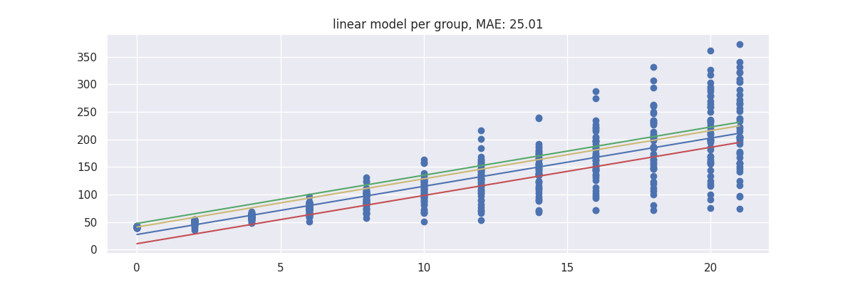
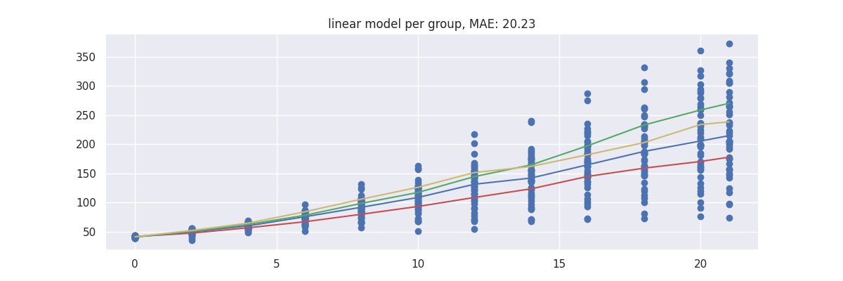
Model 2: Linear Regression in GroupedPredictor

The goal of the GroupedPredictor is to allow us to split up our data.

The image below demonstrates what will happen.

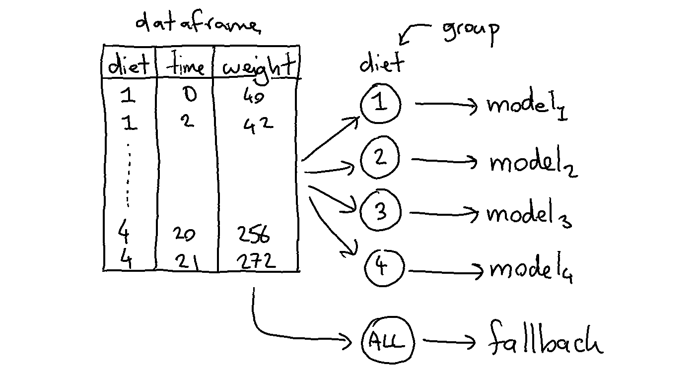
We train 5 models in total because the model will also train a fallback automatically (you can turn this off via use_global_model=False).

The idea behind the fallback is that we can predict something if there is a group at prediction time which is unseen during training.

Each model will accept features that are in X that are not part of the grouping variables. In this case each group will model based on the time since weight is what we're trying to predict.

Applying this model to the dataframe is easy.

GroupedPredictor model

from sklego.meta import GroupedPredictor
mod = GroupedPredictor(LinearRegression(), groups=["diet"])
plot_model(mod)

Such model looks a bit better.

Model 3: Dummy Regression in GroupedEstimation

We could go a step further and train a DummyRegressor per diet per timestep.

The code below works similar as the previous example but one difference is that the grouped model does not receive a dataframe but a numpy array.

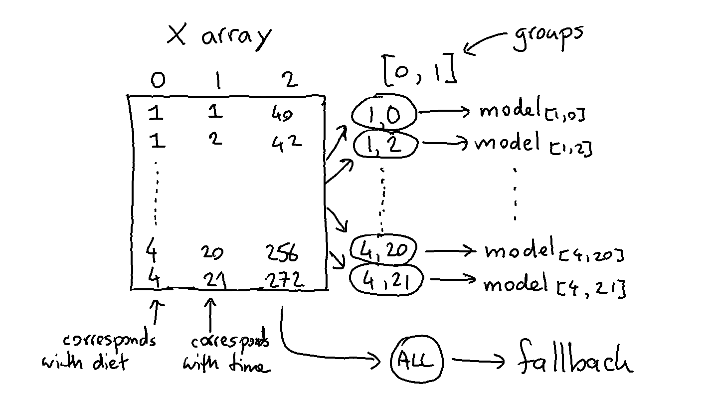
Note that we're also grouping over more than one column here. The code that does this is listed below.

GroupedEstimator with DummyRegressor

from sklearn.dummy import DummyRegressor

feature_pipeline = Pipeline([
    ("datagrab", FeatureUnion([
         ("discrete", Pipeline([
             ("grab", ColumnSelector("diet")),
         ])),
         ("continuous", Pipeline([
             ("grab", ColumnSelector("time")),
         ]))
    ]))
])

pipe = Pipeline([
    ("transform", feature_pipeline),
    ("model", GroupedPredictor(DummyRegressor(strategy="mean"), groups=[0, 1]))
])

plot_model(pipe)

Note that these predictions seems to yield the lowest error but take it with a grain of salt since these errors are only based on the train set.

Specialized Estimators

New in version 0.8.0

Instead of using the generic GroupedPredictor directly, it is possible to work with task specific estimators, namely: GroupedClassifier and GroupedRegressor.

Their specs and functionalities are the exact same of the GroupedPredictor¹ but they are specialized for classification and regression tasks, respectively, by adding checks on the input estimator.

Grouped Transformation

We can apply grouped prediction on estimators that have a .predict() implemented but we're also able to do something similar for transformers, like StandardScaler.

Load penguins

from sklego.datasets import load_penguins

df_penguins = (
    load_penguins(as_frame=True)
    .dropna()
    .drop(columns=["island", "bill_depth_mm", "bill_length_mm", "species"])
)

df_penguins.head()

flipper_length_mm	body_mass_g	sex
181	3750	male
186	3800	female
195	3250	female
193	3450	female
190	3650	male

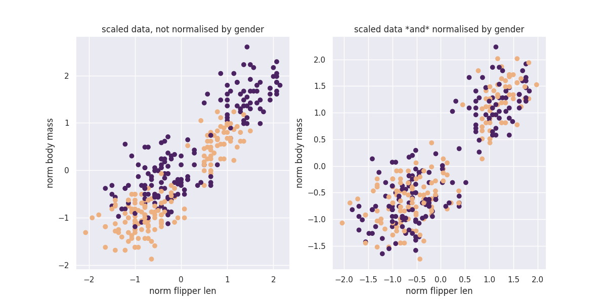
Let's say that we're interested in scaling the numeric data in this dataframe. If we apply a normal StandardScaler then we'll likely get clusters appear for all the species and for the sex. It may be the case (for fairness reasons) that we don"t mind the clusters based on species but that we do mind the clusters based on sex.

In these scenarios the GroupedTransformer can help out. We can specify a grouping column that the data needs to be split on before the transformation is applied.

GroupedTransformer

from sklearn.preprocessing import StandardScaler
from sklego.meta import GroupedTransformer

X = df_penguins.drop(columns=["sex"]).values

X_tfm = StandardScaler().fit_transform(X)
X_tfm_grp = (GroupedTransformer(
    transformer=StandardScaler(),
    groups=["sex"]
    )
    .fit_transform(df_penguins)
)

Code for plotting the transformed data

import matplotlib.pylab as plt
import seaborn as sns
sns.set_theme()

plt.figure(figsize=(12, 6))
plt.subplot(121)

plt.scatter(X_tfm[:, 0], X_tfm[:, 1], c=df_penguins["sex"] == "male", cmap=cmap)
plt.xlabel("norm flipper len")
plt.ylabel("norm body mass")
plt.title("scaled data, not normalised by gender")

plt.subplot(122)
plt.scatter(X_tfm_grp[:, 0], X_tfm_grp[:, 1], c=df_penguins["sex"] == "male", cmap=cmap)
plt.xlabel("norm flipper len")
plt.ylabel("norm body mass")
plt.title("scaled data *and* normalised by gender");

You can see that there are certainly still clusters. These are caused by the fact that there's different species of penguin in our dataset. However you can see that when we apply our GroupedTransformer that we're suddenly able to normalise towards sex as well.

Other scenarios

This transformer also has use-cases beyond fairness. You could use this transformer to causally compensate for subgroups in your data.

For example, for predicting house prices, using the surface of a house relatively to houses in the same neighborhood could be a more relevant feature than the surface relative to all houses.

Hierarchical Prediction

New in version 0.8.0

Very closely related to GroupedPredictor is the HierarchicalPredictor meta estimator and the two task specialized classes HierarchicalClassifier and HierarchicalRegressor.

These estimators fit a separate base estimator for each group in the input data in a hierarchical manner. This means that an estimator is fitted for each subsequential level in the group columns.

Difference with GroupedPredictor

In practice what does that mean? While the APIs are fairly similar, there are a few main differences between hierarchical and grouped meta estimators:

1. The first difference is the fallback method: hierarchical estimators have a fallback method that can be set to either "parent" or "raise". If set to "parent", the estimator will recursively fall back to the parent group in case the group value is not found during .predict().

   Warning

   As a consequence of this, the order of groups matters and potentially a combinatoric number of estimators are fitted, one for each unique combination of group values and each level, including a global one.

2. HierarchicalClassifier is meant to properly handle shrinkage for classification tasks - however this requires that the base estimator implements a .predict_proba() method.

3. While GroupedPredictor is meant to be used directly, HierarchicalPredictor is meant to be used as a base class for other estimators such as HierarchicalClassifier and HierarchicalRegressor.

Shrinkage Functions

Scikit-lego provides a set of shrinkage functions that can be used to shrink the predictions of a model in [Grouped Prediction] and [Hierarchical Predictions].

The following shrinkage are available out of the box:

• "constant": The augmented prediction for each level is the weighted average between its prediction and the augmented prediction for its parent.
• "equal": Each group is weighed equally.
• "min_n_obs": Use only the smallest group with a certain amount of observations.
• "relative": Weigh each group according to its size.

Additionally to the built-in shrinkage functions, it is possible to provide a custom shrinkage function to the GroupedPredictor and HierarchicalPredictor classes.

Such function should takes a list of group sizes and returns an array of the same size with the weights (positive values) for each group.

Custom shrinkage function

import numpy as np

def exp_decay_shrinkage(group_sizes, decay=0.9):
    """A custom shrinkage function that creates an exponential decay which is independent of the group sizes, but
    depends on the decay parameter and the number of groups, and finally normalized to sum to 1.
    """
    a = decay ** np.arange(len(group_sizes), 0, -1)
    return a / a.sum()

exp_decay_shrinkage(group_sizes=[30, 20, 15], decay=0.9)

array([0.29889299, 0.33210332, 0.36900369])

Decayed Estimation

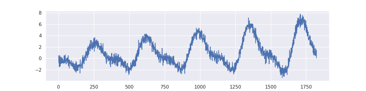
Often you are interested in predicting the future. You use the data from the past in an attempt to achieve this and it could be said that perhaps data from the far history is less relevant than data from the recent past.

This is the idea behind the DecayEstimator meta-model. It looks at the order of data going in and it will assign a higher importance to recent rows that occurred recently and a lower importance to older rows.

Recency is based on the order so it is important that the dataset that you pass in is correctly ordered beforehand.

we'll demonstrate how it works by applying it on a simulated timeseries problem.

TimeSeries data

from sklego.datasets import make_simpleseries

yt = make_simpleseries(seed=1)
df = (pd.DataFrame({"yt": yt,
                   "date": pd.date_range("2000-01-01", periods=len(yt))})
      .assign(m=lambda d: d.date.dt.month)
      .reset_index())

plt.figure(figsize=(12, 3))
plt.plot(make_simpleseries(seed=1));

We will create two models on this dataset. One model calculates the average value per month in our timeseries and the other does the same thing but will decay the importance of making accurate predictions for the far history.

DecayEstimator

from sklearn.dummy import DummyRegressor
from sklego.meta import GroupedPredictor, DecayEstimator

mod1 = (GroupedPredictor(DummyRegressor(), groups=["m"])
        .fit(df[["m"]], df["yt"]))

mod2 = (GroupedPredictor(DecayEstimator(DummyRegressor(), decay_func="exponential", decay_rate=0.9), groups=["m"])
        .fit(df[["index", "m"]], df["yt"]))

plt.figure(figsize=(12, 3))
plt.plot(df["yt"], alpha=0.5);
plt.plot(mod1.predict(df[["m"]]), label="grouped")
plt.plot(mod2.predict(df[["index", "m"]]), label="decayed")
plt.legend();

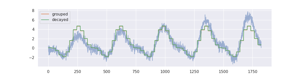
The decay parameter has a lot of influence on the effect of the model but one can clearly see that we shift focus to the more recent data.

Decay Functions

Scikit-lego provides a set of decay functions that can be used to decay the importance of older data. The default decay function used in DecayEstimator is the exponential_decay function (decay_func="exponential").

Out of the box there are four decay functions available:

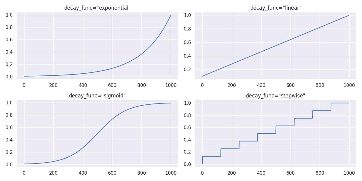
Code for plotting the decay functions

from sklego.meta._decay_utils import exponential_decay, linear_decay, sigmoid_decay, stepwise_decay

fig = plt.figure(figsize=(12, 6))

for i, name, func, kwargs in zip(
    range(1, 5),
    ("exponential", "linear", "sigmoid", "stepwise"),
    (exponential_decay, linear_decay, sigmoid_decay, stepwise_decay),
    ({"decay_rate": 0.995}, {"min_value": 0.1}, {}, {"n_steps": 8})
    ):

    ax = fig.add_subplot(2, 2, i)
    x, y = None, np.arange(1000)
    ax.plot(func(x,y, **kwargs))
    ax.set_title(f'decay_func="{name}"')

plt.tight_layout()

The arguments of these functions can be passed along to the DecayEstimator class as keyword arguments:

DecayEstimator(..., decay_func="linear", min_value=0.5)

To see which keyword arguments are available for each decay function, please refer to the Decay Functions API section.

Notice that passing a string to refer to the built-in decays is just a convenience.

Therefore it is also possible to create a custom decay function and pass it along to the DecayEstimator class, as long as the first two arguments of the function are X and y and the return shape is the same as y:

Custom decay function

def custom_decay(X, y, alpha, beta, gamma):
    """My custom decay function where the magic happens"""
    ...
    return decay_values

DecayEstimator(...,
    decay_func=custom_decay,
    alpha=some_alpha, beta=some_beta, gamma=some_gamma
)

Confusion Balancer

Disclaimer

This feature is an experimental.

We added the ConfusionBalancer as experimental feature to the meta estimators that can be used to force balance in the confusion matrix of an estimator. Consider the following dataset:

Make blobs

import numpy as np
import matplotlib.pylab as plt
import seaborn as sns

sns.set_theme()
cmap=sns.color_palette("flare", as_cmap=True)
np.random.seed(42)

n1, n2, n3 = 100, 500, 50
X = np.concatenate([np.random.normal(0, 1, (n1, 2)),
                    np.random.normal(2, 1, (n2, 2)),
                    np.random.normal(3, 1, (n3, 2))],
                   axis=0)
y = np.concatenate([np.zeros((n1, 1)),
                    np.ones((n2, 1)),
                    np.zeros((n3, 1))],
                   axis=0).reshape(-1)
plt.scatter(X[:, 0], X[:, 1], c=y, cmap=cmap);

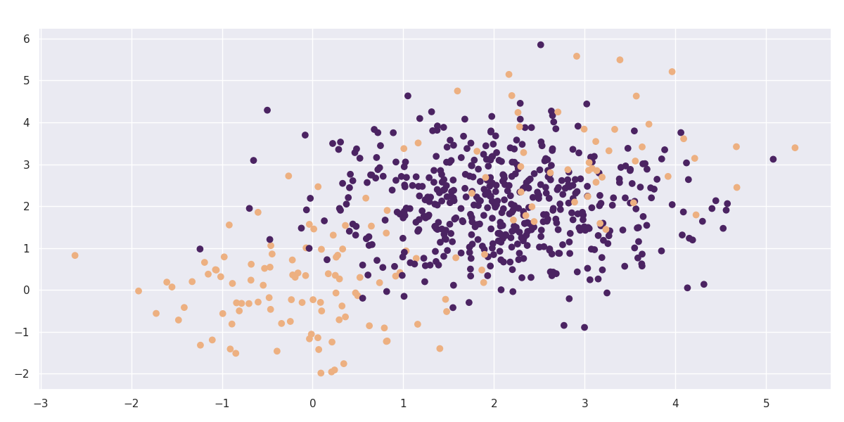
Let's take this dataset and train a simple classifier against it.

from sklearn.metrics import confusion_matrix
from sklearn.linear_model import LogisticRegression

mod = LogisticRegression(solver="lbfgs", multi_class="multinomial", max_iter=10000)
cfm = confusion_matrix(y, mod.fit(X, y).predict(X))
cfm
# array([[ 72,  78],
#        [  4, 496]])

The confusion matrix is not ideal. This is in part because the dataset is slightly imbalanced but in general it is also because of the way the algorithm works.

Let's see if we can learn something else from this confusion matrix. We might transform the counts into probabilities.

cfm.T / cfm.T.sum(axis=1).reshape(-1, 1)
# array([[0.94736842, 0.05263158],
#        [0.1358885 , 0.8641115 ]])

Let's consider the number 0.1359 in the lower left corner. This number represents the probability that the actually class 0 while the model predicts class 1. In math terms we might write this as \(P(C_1 | M_1)\) where \(C_i\) denotes the actual label while \(M_i\) denotes the label given by the algorithm.

The idea now is that we might rebalance our original predictions \(P(M_i)\) by multiplying them;

\[ P_{\text{corrected}}(C_1) = P(C_1|M_0) p(M_0) + P(C_1|M_1) p(M_1) \]

In general this can be written as:

\[ P_{\text{corrected}}(C_i) = \sum_j P(C_i|M_j) p(M_j) \]

In laymens terms; we might be able to use the confusion matrix to learn from our mistakes. By how much we correct is something that we can tune with a hyperparameter.

\[ P_{\text{corrected}}(C_i) = \alpha \sum_j P(C_i|M_j) p(M_j) + (1-\alpha) p(M_j) \]

We'll perform an optimistic demonstration below.

Help functions

def false_positives(mod, x, y):
    return (mod.predict(x) != y)[y == 1].sum()

def false_negatives(mod, x, y):
    return (mod.predict(x) != y)[y == 0].sum()

Confusion Balancer

from sklearn.linear_model import LogisticRegression
from sklearn.model_selection import GridSearchCV
from sklego.meta import ConfusionBalancer

cf_mod = ConfusionBalancer(LogisticRegression(solver="lbfgs", max_iter=1000), alpha=1.0)

grid = GridSearchCV(
    cf_mod,
    param_grid={"alpha": np.linspace(-1.0, 3.0, 31)},
    scoring={
        "accuracy": make_scorer(accuracy_score),
        "positives": false_positives,
        "negatives": false_negatives
    },
    n_jobs=-1,
    return_train_score=True,
    refit="negatives",
    cv=5
)
grid

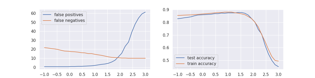
Code to generate the plot

df = pd.DataFrame(grid.fit(X, y).cv_results_)
plt.figure(figsize=(12, 3))

plt.subplot(121)
plt.plot(df["param_alpha"], df["mean_test_positives"], label="false positives")
plt.plot(df["param_alpha"], df["mean_test_negatives"], label="false negatives")
plt.legend()
plt.subplot(122)
plt.plot(df["param_alpha"], df["mean_test_accuracy"], label="test accuracy")
plt.plot(df["param_alpha"], df["mean_train_accuracy"], label="train accuracy")
plt.legend();

It seems that we can pick a value for \(\alpha\) such that the confusion matrix is balanced. there's also a modest increase in accuracy for this balancing moment.

It should be emphasized though that this feature is experimental. There have been dataset/model combinations where this effect seems to work very well while there have also been situations where this trick does not work at all.

It also deserves mentioning that there might be alternative to your problem. If your dataset is suffering from a huge class imbalance then you might be better off by having a look at the imbalanced-learn project.

Zero-Inflated Regressor

There are regression datasets that contain an unusually high amount of zeroes as the targets.

This can be the case if you want to predict a count of rare events, such as defects in manufacturing, the amount of some natural disasters or the amount of crimes in some neighborhood.

Usually nothing happens, meaning the target count is zero, but sometimes we actually have to do some modelling work.

The classical machine learning algorithms can have a hard time dealing with such datasets.

Take linear regression for example: the chance of outputting an actual zero is diminishing.

Sure, you can get regions where you are close to zero, but modelling an output of exactly zero is infeasible in general. The same goes for neural networks.

What we can do circumvent these problems is the following:

1. Train a classifier to tell us whether the target is zero, or not.
2. Train a regressor on all samples with a non-zero target.

By putting these two together in an obvious way, we get the ZeroInflatedRegressor. You can use it like this:

ZeroInflatedRegressor

import numpy as np
from sklearn.ensemble import RandomForestClassifier, RandomForestRegressor
from sklearn.model_selection import cross_val_score
from sklego.meta import ZeroInflatedRegressor

np.random.seed(0)
X = np.random.randn(10000, 4)
y = ((X[:, 0]>0) & (X[:, 1]>0)) * np.abs(X[:, 2] * X[:, 3]**2) # many zeroes here, in about 75% of the cases.

zir = ZeroInflatedRegressor(
    classifier=RandomForestClassifier(random_state=0),
    regressor=RandomForestRegressor(random_state=0)
)

print("ZIR (RFC+RFR) r²:", cross_val_score(zir, X, y).mean())
print("RFR r²:", cross_val_score(RandomForestRegressor(random_state=0), X, y).mean())

ZIR (RFC+RFR) r²: 0.8992404366385873
RFR r²: 0.8516522752031502

Outlier Classifier

Outlier models are unsupervised so they don't have predict_proba or score methods.

In case you have some labelled samples of which you know they should be outliers, it could be useful to calculate metrics as if the outlier model was a classifier.

Moreover, if outlier models had a predict_proba method, you could use a classification model combined with an outlier detection model in a StackingClassifier and take advantage of probability outputs of both categories of models.

To this end, the OutlierClassifier turns an outlier model into a classification model.

A field of application is fraud: when building a model to detect fraud, you often have some labelled positives but you know there should be more, even in your train data.

If you only use anomaly detection, you don't make use of the information in your labelled data set. If you only use a classifier, you might have insufficient data to do proper train-test splitting and perform hyperparameter optimization.

Therefore one could combine the two approaches as shown below to get the best of both worlds.

In this example, we change the outlier model IsolationForest into a classifier using the OutlierClassifier. We create a random dataset with 1% outliers.

OutlierClassifier

import numpy as np
from sklego.meta.outlier_classifier import OutlierClassifier
from sklearn.ensemble import IsolationForest

n_normal = 10_000
n_outlier = 100
np.random.seed(0)
X = np.hstack((np.random.normal(size=n_normal), np.random.normal(10, size=n_outlier))).reshape(-1,1)
y = np.hstack((np.asarray([0]*n_normal), np.asarray([1]*n_outlier)))

clf = OutlierClassifier(IsolationForest(n_estimators=1000, contamination=n_outlier/n_normal, random_state=0))
clf.fit(X, y)

OutlierClassifier(model=IsolationForest(contamination=0.01, n_estimators=1000,
                                        random_state=0))

In a Jupyter environment, please rerun this cell to show the HTML representation or trust the notebook.
On GitHub, the HTML representation is unable to render, please try loading this page with nbviewer.org.

Anomaly detection algorithms in scikit-Learn return values -1 for inliers and 1 for outliers.

As you can see, the OutlierClassifier predicts inliers as 0 and outliers as 1:

OutlierClassifier output

print("inlier: ", clf.predict([[0]]))
print("outlier: ", clf.predict([[10]]))

inlier:  [0.]
outlier:  [1.]

The predict_proba method returns probabilities for both classes (inlier, outlier):

OutlierClassifier predict_proba

clf.predict_proba([[10]])

array([[0.0376881, 0.9623119]])

The OutlierClassifier can be combined with any classification model in the StackingClassifier as follows:

Stacking OutlierClassifier

from sklearn.ensemble import StackingClassifier, RandomForestClassifier

estimators = [
    ("anomaly", OutlierClassifier(IsolationForest())),
    ("classifier", RandomForestClassifier())
    ]

stacker = StackingClassifier(estimators, stack_method="predict_proba", passthrough=True)
stacker.fit(X,y)

StackingClassifier(estimators=[('anomaly',
                                OutlierClassifier(model=IsolationForest())),
                               ('classifier', RandomForestClassifier())],
                   passthrough=True, stack_method='predict_proba')

In a Jupyter environment, please rerun this cell to show the HTML representation or trust the notebook.
On GitHub, the HTML representation is unable to render, please try loading this page with nbviewer.org.

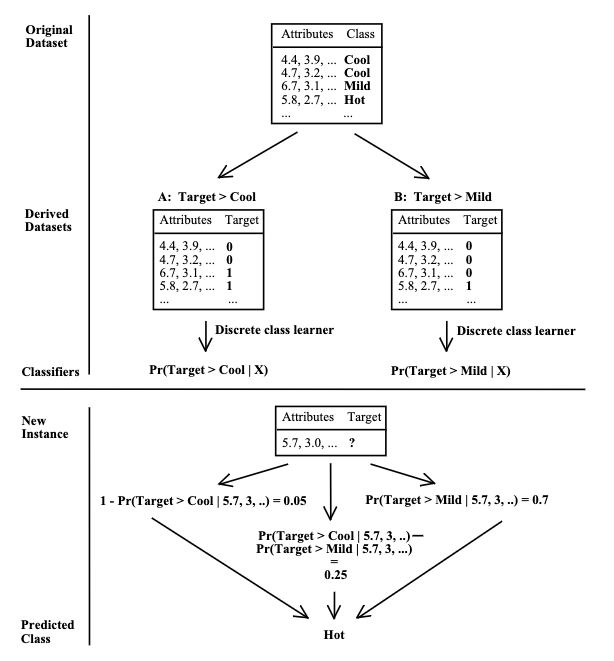
Ordinal Classification

Ordinal classification (sometimes also referred to as Ordinal Regression) involves predicting an ordinal target variable, where the classes have a meaningful order. Examples of this kind of problem are: predicting customer satisfaction on a scale from 1 to 5, predicting the severity of a disease, predicting the quality of a product, etc.

The OrdinalClassifier is a meta-model that can be used to transform any classifier into an ordinal classifier by fitting N-1 binary classifiers, each handling a specific class boundary, namely: \(P(y <= 1), P(y <= 2), ..., P(y <= N-1)\).

This implementation is based on the paper A simple approach to ordinal classification and it allows to predict the ordinal probabilities of each sample belonging to a particular class.

Graphical representation

An image (from the paper itself) is worth a thousand words:

mord library

If you are looking for a library that implements other ordinal classification algorithms, you can have a look at the mord library.

Ordinal Data

import pandas as pd

url = "https://stats.idre.ucla.edu/stat/data/ologit.dta"
df = pd.read_stata(url).assign(apply_codes = lambda t: t["apply"].cat.codes)

target = "apply_codes"
features = [c for c in df.columns if c not in {target, "apply"}]

X, y = df[features].to_numpy(), df[target].to_numpy()
df.head()

apply	pared	public	gpa	apply_codes
very likely	0	0	3.26	2
somewhat likely	1	0	3.21	1
unlikely	1	1	3.94	0
somewhat likely	0	0	2.81	1
somewhat likely	0	0	2.53	1

Description of the dataset from statsmodels tutorial:

This dataset is about the probability for undergraduate students to apply to graduate school given three exogenous variables:

• their grade point average (gpa), a float between 0 and 4.
• pared, a binary that indicates if at least one parent went to graduate school.
• public, a binary that indicates if the current undergraduate institution of the student is > public or private.

apply, the target variable is categorical with ordered categories: "unlikely" < "somewhat likely" < "very likely".

[...]

For more details see the the Documentation of OrderedModel, the UCLA webpage.

The only transformation we are applying to the data is to convert the target variable to an ordinal categorical variable by mapping the ordered categories to integers using their (pandas) category codes.

We are now ready to train a OrdinalClassifier on this dataset:

OrdinalClassifier

from sklearn.linear_model import LogisticRegression
from sklego.meta import OrdinalClassifier

ord_clf = OrdinalClassifier(LogisticRegression(), n_jobs=-1, use_calibration=False)
_ = ord_clf.fit(X, y)
ord_clf.predict_proba(X[0])

[[0.54883853 0.36225347 0.088908]]

Probability Calibration

The OrdinalClassifier emphasizes the importance of proper probability estimates for its functionality. It is recommended to use the CalibratedClassifierCV class from scikit-learn to calibrate the probabilities of the binary classifiers.

Probability calibration is not enabled by default, but we provide a convenient keyword argument use_calibration to enable it as follows:

OrdinalClassifier with probability calibration

from sklearn.calibration import CalibratedClassifierCV
from sklearn.linear_model import LogisticRegression
from sklego.meta import OrdinalClassifier

calibration_kwargs = {...}

ord_clf = OrdinalClassifier(
    estimator=LogisticRegression(),
    use_calibration=True,
    calibration_kwargs=calibration_kwargs
)

# This is equivalent to:
estimator = CalibratedClassifierCV(LogisticRegression(), **calibration_kwargs)
ord_clf = OrdinalClassifier(estimator)

Computation Time

As a meta-estimator, the OrdinalClassifier fits N-1 binary classifiers, which may be computationally expensive, especially with a large number of samples, features, or a complex classifier.

---

1. Not entirely true, as GroupedClassifier doesn't allow for the shrinkage parameter. ↩